Example - Eddy Currents in a Thin-Walled Torus
This example demonstrates the following features of oersted:
- The time-domain eddy current solver and computing resultant forces on a 3D volume
- Computing eddy currents on a geometry with complex homology, without the need for a separate cohomology evaluation
Problem Statement
A conducting thin-walled torus is suspended in a 1 T background field. A circular loop coil is present inside the torus, carrying a current of 100 kA. Over a time period of 10ms, the current in the coil decays, driving eddy currents in the torus. Find the torque acting on the torus due to the interaction between the induced eddy currents and the background field.
- $ \rho= 1.0 \cdot 10^{-7} \space \Omega \cdot m $
- Torus major and minor radii: $ R = 100 \space mm, a = 20 \space mm $
- Torus wall thickness: $ t = 10 \space mm $
- Cross-field: $ B_x = 1 \space T $
- Coil current and decay time: $ I_0 = 100 \space kA, t_{ramp} = 10 \space ms $
- Both the torus and the ring coil are aligned with the z-axis
Create Geometry
The testing module in oersted provides simple means of accessing the gmsh API to
create geometry primitives.
Torus:
major_radius = 0.10 # (m)
minor_radius = 0.02 # (m)
wall_thickness = 0.01 # (m)
mesh_size = 0.01 # (m)

torus: Mesh = oersted.testing.make_torus(
    major_radius, minor_radius, wall_thickness, mesh_size
)
Ring coil:
initial_current = 1e5 # (A)
z_height = 0.0
width = 0.005 # (m) cross-section
height = 0.005 # (m)
ring_jmag = initial_current / (width * height) # (A/m^2)
mesh_size = width
ring, ring_jdensity = oersted.testing.make_ring(
    major_radius, z_height, width, height, mesh_size, jmag=ring_jmag
)
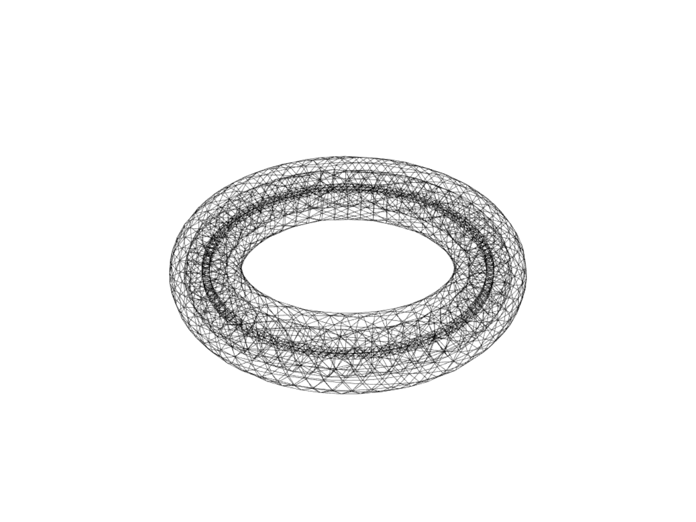
Plot both meshes:
mesh = torus.append(ring)
oersted.mesh.plot(mesh, transparency=True)
Compute Driven Coil Excitations
The transient solver in oersted attempts to be completely agnostic of how the external
changing fields are generated. To do this, it assumes that the driven coils are
unaffected by the passive components. This way, external changing fields can be
generated any way the user needs.
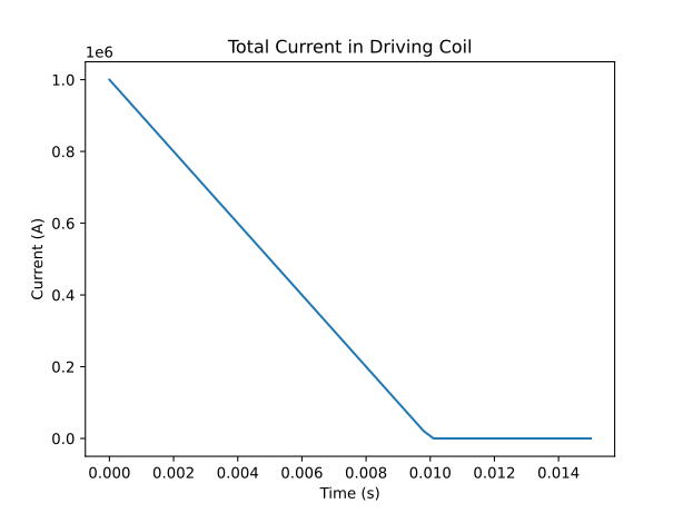
In this example, the external fields are easy to compute; simply create a linear ramp in time, then scale the fields generated by the ring at maximum current:
# Time properties: linear decay to zero in 10ms, then watch the eddy currents decay
nt = 50
t_end = 0.015  # (s)
t_ramp = 0.010  # (s)
time = np.linspace(0, t_end, nt)
scale = np.maximum(1.0 - time / t_ramp, 0.0)

# Compute external fields acting on the torus (from the ring coil) over time
a_ext = np.zeros((nt, torus.num_elems, 3))
b_ext = np.zeros((nt, torus.num_elems, 3))

# A and B fields at maximum coil current, using the ring and its elemental current
# density at maximum current as the source
a_unit = oersted.a_field(ring, torus.centroids, jdensity=ring_jdensity)
b_unit = oersted.b_field(ring, torus.centroids, jdensity=ring_jdensity)

# Scale the fields to produce a simple linear decay over time
a_ext = scale[:, None, None] * a_unit
b_ext = scale[:, None, None] * b_unit
Solve and Compute Torque
The eddy current solver (in its present form) assumes that the mesh is continuous and is made of the same material (this will change in future releases). Therefore, running the solution is as simple as passing the mesh information, the resistivity of the material, the time properties, and the external fields:
results = oersted.transient_solve(torus, rho, nt, t_end, a_ext, b_ext)
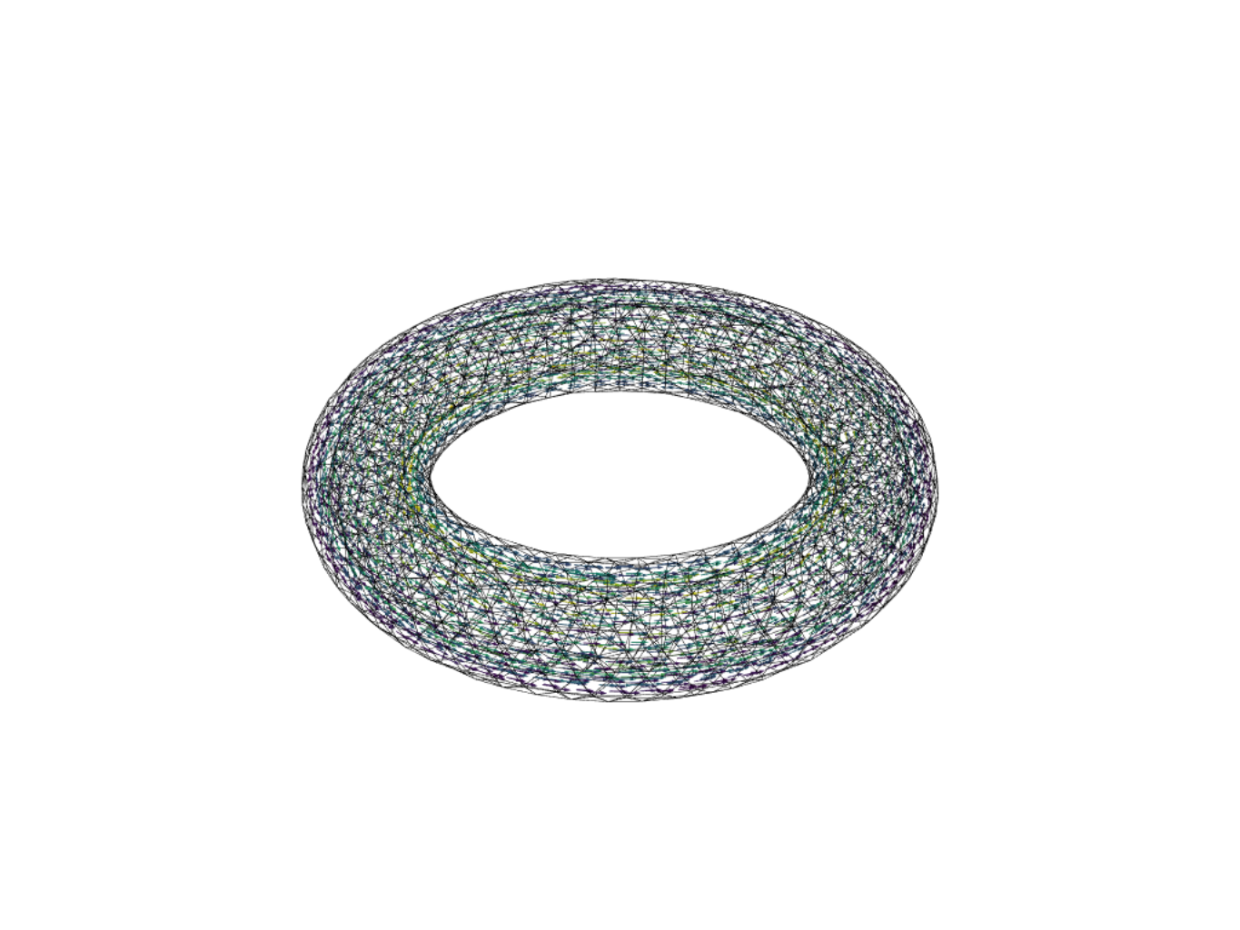
Eddy currents in the torus at the end of the coil ramp:
Compute torque about centroid of torus, which is the origin:
# f = j x b
f = np.cross(results.j, cross_field) * torus.volumes[None, :, None]

# T = sum(r x f)
torque = np.sum(np.cross(torus.centroids[None, :, :], f), axis=1)
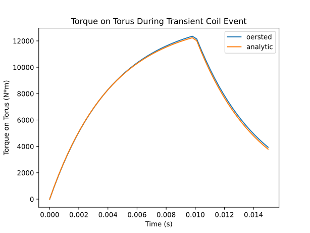
Torque can also be estimated by considering an L/R circuit of the same system, which
shows good agreement against the oersted solution: